Note
Go to the end to download the full example code.
ASM1: confounding on the inflection points of the S_O#
# Copyright (C) 2024 Juan Pablo Carbajal
# Copyright (C) 2024 Mariane Yvonne Schneider
#
# This program is free software; you can redistribute it and/or modify
# it under the terms of the GNU General Public License as published by
# the Free Software Foundation; either version 3 of the License, or
# (at your option) any later version.
#
# This program is distributed in the hope that it will be useful,
# but WITHOUT ANY WARRANTY; without even the implied warranty of
# MERCHANTABILITY or FITNESS FOR A PARTICULAR PURPOSE.  See the
# GNU General Public License for more details.
#
# You should have received a copy of the GNU General Public License
# along with this program. If not, see <http://www.gnu.org/licenses/>.

# Author: Juan Pablo Carbajal <ajuanpi@gmail.com>
# Author: Mariane Yvonne Schneider <myschneider@meiru.ch>
import matplotlib.pyplot as plt
import numpy as np
import pandas as pd
from scipy.integrate import solve_ivp
from sympy import *

try:
    import dsafeatures
except ModuleNotFoundError:
    import sys
    import os

    sys.path.insert(0, os.path.abspath("../.."))

import dsafeatures.odemodel as m
import dsafeatures.symtools as st
import dsafeatures.signal_processing as sp
import dsafeatures.analysis as an
import dsafeatures.interactive as gui

from dsafeatures.printing import *
init_printing()
Load the model#
asm = m.ODEModel.from_csv(name="ASM1")
# States
X = asm.states
# Process rates
r_sym, r = asm.rates, asm.rates_expr
Jr = r.jacobian(X)
# Matrix
M = asm.coef_matrix
# State derivative
dotX = asm.derivative()

O2, idxO2 = asm.state_by_name("S_O2")
Aeration#
Define aeration
Inflection point curve#
Parameter values#
param_values = dict(asm.parameters(and_values=True).set_index("sympy").value)
param_values = {k: v.subs(param_values) for k, v in param_values.items()}
replace parameter symbols with values
ipc_pv = ipc.subs(zip(r_sym, r)).subs(param_values).doit()
ipc_pv
Find on which states the IPC depends on
ipc_states = sorted(tuple(x for x in X if ipc.has(x)), key=str)
ipc_states
[S_\text{NHx}, S_\text{NOx}, S_\text{O2}, S_\text{bN}, S_\text{b}, X_\text{a}, X_\text{cb}, X_\text{h}]
same for ODE system
dotX_pv = dotX.subs(zip(r_sym, r)).subs(param_values).doit()
dO2dt_states = sorted(tuple(x for x in X if dotX_pv[idxO2].has(x)), key=str)
dO2dt_states
[S_\text{NHx}, S_\text{O2}, S_\text{b}, X_\text{a}, X_\text{h}]
states_to_set = sorted(list(set(ipc_states) | set(dO2dt_states)), key=str)
Numerical check#
State values initial values
states_iv = asm.component["states"][["sympy", "initial_value"]].set_index("sympy").loc[list(X), "initial_value"]
Integrate numerically
Spline representation
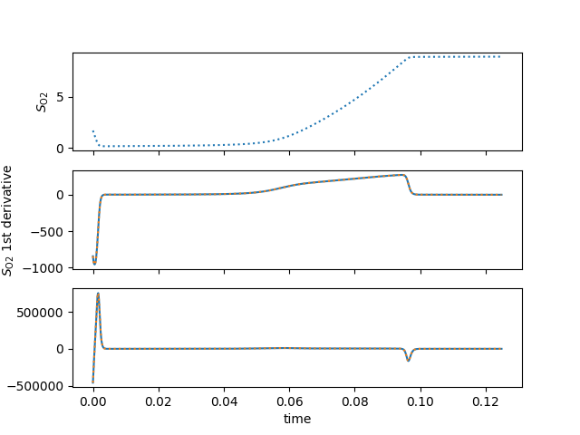
fig, axs = plt.subplots(nrows=3, sharex=True)
ax = axs[0]
ax.plot(t, y[idxO2], ':', label="numerical")
ax.set_ylabel(latex(O2, mode="inline"))

ax = axs[1]
ax.plot(t, dx_val, label="symbolic")
ax.plot(t, dx_s(t), ':', label="numerical")
ax.set_ylabel(latex(O2, mode="inline")+" 1st derivative")

ax = axs[2]
ax.plot(t, ipc_val, label="symbolic")
ax.plot(t, ipc_s(t), ':', label="numerical")
ax.set_ylabel(latex(O2, mode="inline")+" 2nd derivative")
ax.set_xlabel("time")
Analysis#
%% Set limits for O2
Set value for NHx
NHx, idxNHx = asm.state_by_name("S_NHx")
Find zeros of ipc for all states with random values
# minimum value for derivative
dotO2_min = 4e-2
# initialize random generator
rng = np.random.default_rng(list(map(ord, "abracadabra")))
# initial values of states to set
states_iv = asm.component["states"][["sympy", "initial_value"]].set_index("sympy").loc[states_to_set, "initial_value"]
nsamples = 100
samples = pd.DataFrame(columns=states_to_set, dtype=float)
for Y in states_to_set:
if Y == NHx:
samples.loc[:, Y] = rng.uniform(low=1.0, high=200.0, size=nsamples)
else:
samples.loc[:, Y] = rng.uniform(low=1e-3, high=min(max(states_iv[Y] * 10, 10), 5e3), size=nsamples)
if "hits" not in locals():
hits = dict()
ngrid = 60
# normalized grid
g1, g2 = np.meshgrid(*(np.linspace(0, 1, ngrid), )*2)
# grid for oxygen
xx = g1 * (O2_limits[2] - O2_limits[1]) + O2_limits[1]
# oxygen derivative
dotO2 = dotX_pv[idxO2]
for Y in states_to_set:
if Y == O2:
continue
# grid for Y state, default estimated maximum
ymax = max(20, 3 * states_iv[Y])
yy = g2 * ymax
other_states = tuple(s for s in states_to_set if s not in (O2, Y))
q, vv = an.masked_contours2d(ipc_pv, vars=(O2, Y), params=other_states,
vars_grid=(xx, yy), params_samples=samples.loc[:, list(other_states)].to_numpy(),
maskfunc=[(dotO2, dotO2_min)])
if vv:
ql = np.vstack([l_ for q_ in q for l_ in q_])
yrng = (ql[:, 1].min(), ql[:,1].max())
hits[Y] = {"states": other_states, "samples": np.asarray(vv), "contours": q, "range": yrng}
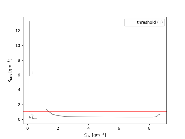
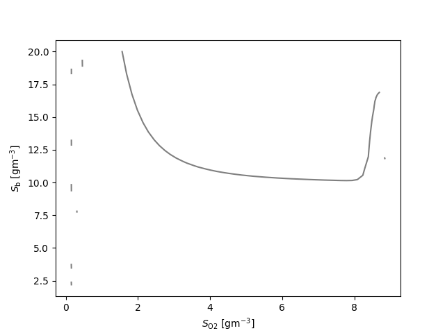
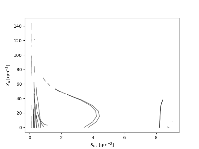
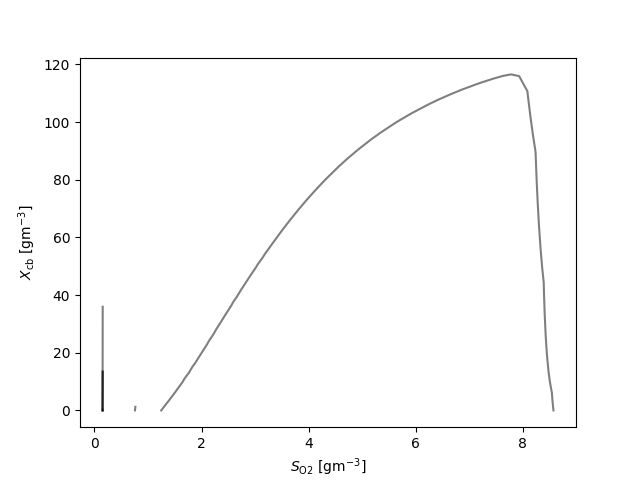
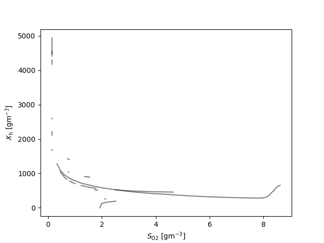
fig, ax = plt.subplots()
for q_ in q:
for l_ in q_:
ax.plot(l_[:,0], l_[:,1], 'k', alpha=0.5)
ax.set_xlabel(latex(O2, mode='inline')+' [g$\mathrm{m}^{-3}$]')
ax.set_ylabel(latex(Y, mode='inline')+' [g$\mathrm{m}^{-3}$]')
if Y == NHx:
plt.axhline(y=1.0, color='r', linestyle='-', label='threshold (T)')
plt.legend()
/builds/sbrml/dsa-signal-features/doc/examples/example_asm1_SO_inflection_confounding.py:208: SyntaxWarning: invalid escape sequence '\m'
  ax.set_xlabel(latex(O2, mode='inline')+' [g$\mathrm{m}^{-3}$]')
/builds/sbrml/dsa-signal-features/doc/examples/example_asm1_SO_inflection_confounding.py:209: SyntaxWarning: invalid escape sequence '\m'
  ax.set_ylabel(latex(Y, mode='inline')+' [g$\mathrm{m}^{-3}$]')
The numer of random samples of the states values that generated an ipc
{S_\text{NHx}: 7, S_\text{b}: 7, X_\text{a}: 19, X_\text{cb}: 6, X_\text{h}: 10}
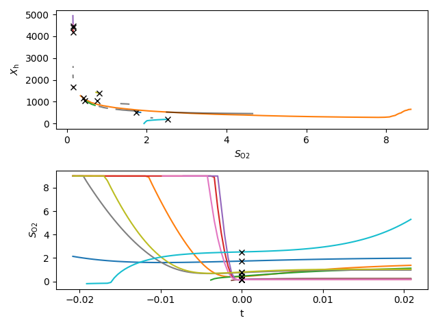
Trajectory of point in ipc#
ODE definition
args_ = an.numeric_ode(dotX_pv, list(X), ub={O2: maxO2})
Tmax = 30.0 / 1440

def ev(t, y, dir=1.0):
    return ipc_np(y)
ev.terminal = 0
ev.direction = -1

args_ = args_ | dict(t_span=(0, Tmax),
                     first_step=1e-8,
                     max_step=1e-3,
                     t_eval=np.linspace(0, Tmax, 50),
                     method="Radau",
                     events=[ev])
Select plane y_state = sorted(hits, key=lambda k: max([y.allsegs[0][0][:,0].max()-y.allsegs[0][0][:,0].min() for y in hits[k][“contours”]]))[0] y_state = NHx y_state = context[“states”][“X_ANO”]
y_state, idxy = asm.state_by_name("X_OHO")

# initial values
iv_def = asm.component["states"][["sympy", "initial_value"]].set_index("sympy")["initial_value"]
iv_def = np.maximum(iv_def, 1.0)  # avoid 0 initial values

f, axs = plt.subplots(nrows=2, tight_layout=True)
axs[0].set_xlabel(latex(O2, mode='inline'))
axs[0].set_ylabel(latex(y_state, mode='inline'))
axs[1].set_xlabel('t')
axs[1].set_ylabel(latex(O2, mode='inline'))
lgd = []
for q, idx_sample in zip(hits[y_state]["contours"], hits[y_state]["samples"]):
    # get point on ipc
    qmid = (2, 1200)
    dmin = np.inf
    pxy = []
    cidx = -1
    for ci, c in enumerate(q):
        d_ = ((c - qmid)**2).sum(axis=1)
        idx = np.argmin(d_)
        if d_[idx] < dmin:
            dmin = d_[idx]
            pxy = c[idx]
            cidx = ci
    ptx, pty = pxy

    # integrate ODE

    # Generate initial value
    iv = iv_def.copy()
    iv_ = samples.loc[idx_sample].copy()
    iv.loc[iv_.index] = iv_
    iv[O2] = ptx
    iv[y_state] = pty
    iv_ls = iv[list(X)].to_list()

    sol = solve_ivp(**args_, y0=iv_ls)
    sol_r = solve_ivp(**args_, y0=iv_ls, args=(-1.0,))

    ax = axs[0]
    for ci, c in enumerate(q):
        if ci == cidx:
            ax.plot(c[:, 0], c[:, 1])
            clc = ax.get_lines()[-1].get_color()
        else:
            ax.plot(c[:, 0], c[:, 1], color="k", alpha=0.5)
    ax.plot(ptx, pty, 'xk')

    ax = axs[1]
    ax.plot(sol.t, sol.y[idxO2], color=clc)
    ax.plot(-sol_r.t, sol_r.y[idxO2], color=clc)
    ax.plot(0, ptx, 'xk')
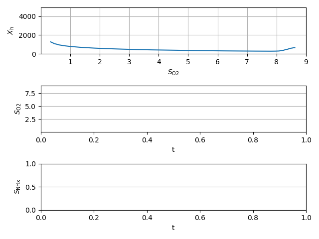
Interactive#
After all the plots a new interactive plot appears This si not interactive in the example
# find sample with contour with max length
lmax = -np.inf
imax = 0
for i, q in zip(hits[y_state]["samples"], hits[y_state]["contours"]):
    for c in q:
        # approx. length
        lc = np.sum(np.sqrt(np.sum(np.diff(c, axis=0)**2, axis=1)))
        if lc > lmax:
            lmax = lc
            imax = i
qmax = hits[y_state]["samples"].tolist().index(imax)

# Generate initial value
iv = iv_def.copy()
iv_ = samples.loc[imax].copy()
iv.loc[iv_.index] = iv_
iv = iv[list(X)].to_list()

# plot these contours
f, axs = plt.subplots(nrows=3, tight_layout=True)
axs[0].set_xlabel(latex(O2, mode='inline'))
axs[0].set_ylabel(latex(y_state, mode='inline'))
axs[1].set_xlabel('t')
axs[1].set_ylabel(latex(O2, mode='inline'))
axs[2].set_xlabel('t')
axs[2].set_ylabel(latex(NHx, mode='inline'))

ax = axs[0]
for c in hits[y_state]["contours"][qmax]:
    ax.plot(c[:, 0], c[:, 1])
# start interactive plot
Xlist = list(X)
gui.interactive_ipc_ode(O2_limits, (y_state, *hits[y_state]["range"]), Xlist, dotX_pv, iv,
                        also_show=[NHx],
                        fig=f)

plt.show()
Total running time of the script: (0 minutes 10.041 seconds)
Estimated memory usage: 239 MB